
Practical guide · Base R
Published
Single-arm trials: response and denominators
Audit a response proportion before interpreting it: reconstruct counts, calculate uncertainty and check what changes when unknown outcomes are excluded.
Download the R scriptSee the stepsRead the news article and regulatory context
- Save the script in your own folder.
- Open it in RStudio and run source("response-denominators.R").
- Run run_exercise("downloads"); read the results and limitations below.
28 people. Two denominators.
Documented response duration of at least 12 months, in the CIS efficacy population.
Among responders
28 / 4858.3%
Over the initial CIS cohort
28 / 7736.4%
We use two separate materials: public FDA aggregate counts for Anktiva’s CIS population and an entirely synthetic exercise involving 100 people. No file contains individual trial records. The purpose is descriptive and educational; we do not evaluate a clinical indication or compare treatments.
1. Define the quantity before opening R
The unit is the person. A binary response needs a numerator, a denominator and an assessment rule. Response at any time and response at the six-month visit are different variables, even when both use zero and one. Eligibility, the visit schedule and treatment of rescue therapy, deaths and missing assessments also need to be defined. A valid numeric column does not establish its scientific meaning.
In this exercise, x is the response count and n the number of people in the relevant population. There are no predictors or covariate adjustments: we calculate a descriptive proportion and a binomial interval. Interpretation as a common probability requires independent observations under the chosen model. Repeated visits, centre clustering or different opportunities to respond may require another analysis.
The synthetic dictionary contains id, a unique identifier prefixed SYN, and response: 1 means documented response at the teaching horizon, 0 documented non-response, and a blank cell an unknown outcome. All 100 people belong to the population defined before observing outcomes. They are separate from Anktiva’s 77-person efficacy population.
2. Reproduce a published aggregate estimate
The FDA Snapshot reports 48 responses among 77 people with CIS, with or without papillary disease. We use the count to audit arithmetic. We do not attribute it to the papillary-only population added in October or reconstruct individual records from the aggregate totals.
source("response-denominators.R")


response_summary(48, 77)


stats::binom.test(48, 77, conf.level = 0.95)$conf.int
The result is a proportion of 0.6233766, with limits of 0.5056248 and 0.7313324: 62.34% and a 95% interval of 50.56% to 73.13%. The function uses Clopper–Pearson. Coverage is at least nominal under the binomial model and can be conservative. The interpretation is frequentist: the procedure has a repeated-sampling coverage property; it does not assign 95% probability to this fixed parameter. Official R documentation.
The interval quantifies one source of uncertainty. It does not repair selective recruitment, informative missingness or outcome misclassification. Nor does it estimate a difference against an absent control. Although binom.test returns a p-value, we extract only the interval: we have not defined a clinically justified historical threshold for a hypothesis test.
3. Check what changes with the denominator
The published duration counts are 28 and 19, using the 48 responders as denominator. Their relationship to all 77 people can be calculated arithmetically while retaining each row’s meaning. The fda-denominators.csv file preserves numerator, denominator, proportion and provenance. Derived rows are identified as our descriptive calculations.
48 / 77                 # response at any time


28 / 48                 # duration >=12 months among responders


19 / 48                 # duration >=24 months among responders


(48 / 77) * (28 / 48)    # exactly 28/77


28 / 77                 # documented count over the initial population
The last result is 36.36%. It should not be called disease-free survival at 12 months from treatment initiation. The duration clock starts at response, potentially at different visits for different people. A documented count also does not adjust for censoring or insufficient observation time. The algebra remains correct, but the scientific name must match what was calculated.
For duration analysis using individual data, define the event, time origin and censoring rules. Death may be part of the endpoint or a competing event depending on the question; it does not automatically become independent censoring. The published Kaplan–Meier guide develops time, censoring and numbers at risk. We do not invent an Anktiva curve to complete this exercise.
4. Separate precision from magnitude
Synthetic samples of 20, 80 and 200 people have exactly 60% response: 12, 48 and 120 responses respectively. Their exact intervals differ. A larger denominator adds precision under the same model without making a descriptive estimate causal. These are separate scenarios, not three successive analyses of accumulating follow-up.
| Response / total | Response (%) | Exact 95% CI (%) |
|---|---|---|
| 12 / 20 | 60.0 | 36.05 – 80.88 |
| 48 / 80 | 60.0 | 48.44 – 70.80 |
| 120 / 200 | 60.0 | 52.85 – 66.85 |
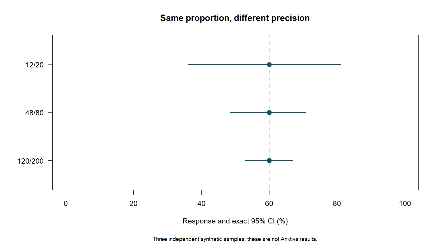
The chart retains a 0–100% scale to avoid exaggerating changes in interval width. It represents neither the probability that a particular patient responds nor a ranking of studies by efficacy. Comparing populations or interventions requires appropriate design and an estimand as well as an interval.
5. Explore ten unknown responses
The synthetic CSV contains 60 responses, 30 non-responses and 10 unknown values. The observed-outcome proportion is 60/90 = 66.67%. This describes people with recorded outcomes. It does not automatically represent all 100 because the operation removes blank values without producing an error.
d <- read.csv("downloads/synthetic-response.csv")


mean(d$response, na.rm = TRUE)


missing_scenarios(d$response)
The function keeps all 100 people in the denominator and successively assigns zero through ten responses to unknown outcomes. It produces eleven completions, from 60/100 to 70/100. The 60–70% range bounds the completed proportion in this sample. It is not a confidence interval, multiple imputation or a statement that all completions are equally probable.
MCAR, MAR and MNAR describe different assumptions about missingness. This exercise does not identify which holds. Interpreting complete cases as an estimate for the original population requires justification of the mechanism and the relevant conditions. Assigning every unknown to non-response may be a conservative rule for a specific variable, but it must be defined; it does not demonstrate that the unobserved outcomes really were negative.
6. Avoid an improvised historical comparison
Suppose you find an earlier study reporting 40% response. Subtracting it from 62.34% does not identify a causal benefit of 22.34 percentage points. Populations, definitions, visits, prior resection and missing-data handling may differ. Even the denominator might include people who would not meet eligibility rules in the current study.
An external comparison needs its own protocol: shared eligibility, time origin, a confounding strategy and sensitivity analyses. Adjustment for observed variables does not guarantee absence of residual confounding. We calculate no risk ratio, NNT or treatment superiority here because the available counts do not support those estimates. The FDA guidance on oncology endpoints places design and outcome choice in context.
7. Run the exercise and retain provenance
Download the script to your own folder, open it in RStudio and run the following commands from that folder. It installs no packages and does not alter your input data. It writes known output filenames to the directory you specify; choose a new directory if you want to preserve an earlier run.
source("response-denominators.R")


run_exercise("downloads")


d <- read.csv("downloads/synthetic-response.csv")


response_summary(sum(d$response == 1, na.rm = TRUE),


                 sum(!is.na(d$response)))


range(missing_scenarios(d$response)$estimate)Outputs are deterministic: no random simulation or seed needs to be recovered. The script uses base R and the bundled stats, graphics and grDevices packages. The sessionInfo.txt record captures the R version actually run. FDA files contain derived aggregates; SYN identifiers belong only to the synthetic exercise. Never merge the two origins into a patient dataset.
8. Four worked exercises
1. Does 58% mean durable response in 58% of all 77 people?
No. The published denominator is 48 responders: 28/48 = 58.33%. Over all 77 people, the documented count is 28/77 = 36.36%. This transformation provides neither a Kaplan–Meier duration estimate nor response at a fixed visit from treatment initiation.
2. Why do 12/20 and 120/200 have different intervals?
Both give 60%, but sample sizes differ. Run response_summary(12,20) and response_summary(120,200). The second interval is narrower under the binomial model. Neither on its own establishes comparative efficacy or transportability.
3. What if eight of the ten unknown outcomes were responses?
The completed sample has 68 responses among 100 people: 68%. Locate missing_responders_assumed == 8 in the sensitivity CSV. This is an explicit assumption, not an observed result. Complete cases still give 66.67%, because they answer a different question.
4. Can 48/77 be used as an observed rate for the new papillary population?
No. The aggregate comes from the CIS population. The regulatory expansion relies on an extrapolation argument; it does not retrospectively change the population supplying this count. A correct table retains population, source, definition and date.
9. Write an auditable result
A useful statement would read: “In the FDA-described CIS efficacy population, 48 of 77 people achieved complete response at any time; our recalculated proportion is 62.34%, with exact 95% binomial confidence interval 50.56–73.13%. There is no comparator arm in this aggregate.” Report duration separately with its own denominator.
For your project, keep outcome definitions, missing-data rules and cutoff dates in the dictionary. If a decision changes after results are seen, record it as a subsequent decision and assess its impact against the original specification. A reproducible run helps audit what you did; scientific validity also requires justification that the calculation answers the question.